PurposeMeasure a cart’s momentum change and compare to the impulse it receives.
Compare average and peak forces in impulses. |
Materials
|
PROCEDURE
1. Measure the mass of your dynamics cart and record the value in the Data Table.
2. Place the track on a level surface. Confirm that the track is level by placing the low-friction
cart on the track and releasing it from rest. It should not roll. If necessary, adjust the track.
3. Attach the elastic cord to the cart and then the cord to the force sensor. Choose a cord length
so that the cart can roll freely with the cord slack for most of the track length, but be stopped
by the cord before it reaches the end of the track. Clamp the Force Sensor so that the cord,
when taut, is horizontal and in line with the cart’s motion.
4. Place the Motion Detector beyond the other end of the track so that the detector has a clear
view of the cart’s motion along the entire track length. When the cord is stretched to
maximum extension the cart should not be closer than 0.4 m to the detector.
5. Connect the Student Force Sensor to Channel 1 of the CBL 2 interface. Connect the Motion
Detector to the SONIC/DIG or SONIC/DIG 1 input of the interface. Use the black link cable to
connect the interface to the TI Graphing Calculator. Firmly press in the cable ends.
6. Turn on the calculator and start the DATAMATE program. Press CLEAR to reset the program.
7. If CH 1 displays the Force Sensor and its current reading, skip the remainder of this step. If
not, set up DATAMATE for the Force Sensor manually (the interface will recognize the Motion
Detector automatically). To do this,
a. Select SETUP from the main screen.
b. Press ENTER to select CH1
c. Choose FORCE from the SELECT SENSOR list.
d. Choose STUDENT FORCE for your force sensor.
e. Select OK to return to the main screen.
8. Zero the Force Sensor.
a. Select SETUP from the main screen.
b. Select ZERO.
c. Select CH 1 from the SELECT CHANNEL menu.
d. Remove all force from the Force Sensor.
e. When the reading on the calculator screen is stable, press ENTER to record the zero
condition.
9. Set up the calculator and interface for data collection.
a. Select SETUP from the main screen.
b. Press to select MODE and press ENTER .
c. Select TIME GRAPH from the SELECT MODE screen.
d. Select CHANGE TIME SETTINGS.
e. Enter “0.02” as the time between samples in seconds. (Use “0.05” for the TI-73 and 83.)
f. Enter “150” as the number of samples. (Use “50” for the TI-73 and 83.)
g. Select OK twice to return to the main screen.
10. Practice releasing the cart so it rolls toward the Motion Detector, bounces gently, and returns
to your hand. The Force Sensor must not shift and the cart must stay on the track. Arrange the
cord and string so that when they are slack they do not interfere with the cart motion. You
may need to guide the string by hand, but be sure that you do not apply any force to the cart
or Force Sensor. Keep your hands away from between the cart and the Motion Detector.
11. Select START to take data. As soon as you hear the interface beep, roll the cart as you
practiced in the previous step.
12. Study your graphs to determine if the run was useful:
a. Press ENTER to see the force graph.
b. Inspect the force data. If the peak is flattened, then the applied force is too large. Repeat
your data collection with a lower initial speed.
c. Press ENTER to return to the graph selection screen.
d. Press to select DIG-DISTANCE.
e. Press ENTER to see the distance graph.
f. Confirm that the Motion Detector detected the cart throughout its travel. If there is a noisy
or flat spot near the time of closest approach, then the Motion Detector was too close to
the cart. Move the Motion Detector away from the cart, and repeat your data collection.
g. Press ENTER to return to the graph selection screen, and select MAIN SCREEN.
h. To collect further data, return to Step 11.
13. Once you have made a run with good distance and force graphs, analyze your data. To test the
impulse-momentum theorem, you need the velocity before and after the impulse. To find
these values,
a. Select ANALYZE from the main screen.
b. Select STATISTICS from the ANALYZE OPTIONS.
c. Select DIG-VELOCITY from the SELECT GRAPH screen.
d. Now you can select a portion of the velocity graph for averaging. Using the and
cursor keys, move the lower bound cursor to the left side of the approximately constantand negative-velocity region. Press ENTER .
e. Now set the upper bound: Move the cursor to the right edge of the approximately
constant- and negative-velocity region. Press ENTER .
f. Read the average velocity before the collision (vi) from the calculator. Record the value in
your Data Table.
g. Press ENTER to return to the ANALYZE OPTIONS screen.
h. In the same manner, determine the average velocity just after the bounce (vf) and record
this positive value in your Data Table.
14. (Calculus version) Now record the value of the impulse.
a. Select INTEGRAL from the ANALYZE OPTIONS.
b. Select CH1-FORCE(N) from the select graph screen.
c. Now you can select a portion of the force graph for integration. Using the cursor keys,
move the cursor to just before the impulse begins, where the force becomes non-zero.
Press ENTER .
d. Now move the cursor to the right edge of the impulse, where the force returns to zero.
Press ENTER .
e. Calculus tells us that the expression for the impulse is equivalent to the integral of the
force vs. time graph, or
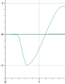
Data
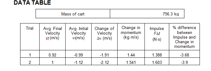
Trial One
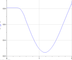
Distance vs Time
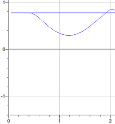
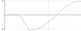
Velocity vs Time
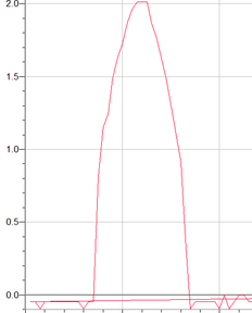
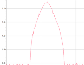
Force vs Time
Trial 2
Distance vs Time
Velocity vs Time
Force vs Time
Data Analysis
The purpose of the lab was to determine the real life application of the equality of change in momentum and the impulse. The percent difference* we achieved in each trial was within 5% both times.
*Percent difference was calculated by dividing the difference between the two values by the average of the two, and then multiply by 100%.
Trial 1: 3.68%
Trial 2: 3.9%
This percent difference can be accounted for by inaccuracies in the equipment. In particular, our force sensor measured a nearly negligible negative force when it should have been zero because of a malfunction in the equipment. This single error in equipment may have been the most significant factor in widening the inequality of the change in momentum versus the impulse.
Because the negative force would have added area below the curve when there should have been none, the integral of the force vs time equation would have had a lower value than the actual impulse. This means that the actual impulse would have a slightly higher value, bringing it closer to the change in momentum calculated above.
The second objective of the lab was to compare average force vs peak force in an impulse. The peak force in an impulse is obtained from the graph of the equation. The average force is obtained by dividing the impulse by the time that the force was applied. The average and peak forces for each trial are:
Trial 1
Peak: 2.01
Avg: 1.388
Trial 2
Peak: 2.26
Avg: 1.78
The impulse in Trial 2 occurred for 0.9 seconds, while Trial one had an impulse lasting 1.0 seconds. This affects the average force in that, the lower the value of time for which an impulse occurs, the greater the force will be for equivalent impulses. Peak force however is independent of time.
Conclusion
Our purpose in this lab was to compare in a real life setting impulse and change in momentum. Our theory would indicate that, without any additional external factors, the two are equal. In practice, we found values that were well within 5% of each other for each trial. This is close enough to say that the theory is conclusive, given that we were unable to perform the experiment in ideal conditions. Some of the conditions that would increase the percent difference in our experiment were faulty equipment that was unable to perfectly zero for force value. That was the most outstanding experimental flaw. Another would be the force dissipated by friction, which was almost negligible in the setup, but was still unaccounted for.
Another purpose of the lab was to compare peak and average forces. The conclusion that can be made here is that peak force is measurable directly from the graph while average force must be calculated by dividing the magnitude of the impulse by the time it was applied. This would lead to the conclusion that peak force is independent of time while average force is not.
Another purpose of the lab was to compare peak and average forces. The conclusion that can be made here is that peak force is measurable directly from the graph while average force must be calculated by dividing the magnitude of the impulse by the time it was applied. This would lead to the conclusion that peak force is independent of time while average force is not.
